2.1Introduction
On October 15, 1997, the Cassini-Huygens spacecraft was launched by NASA’s Jet Propulsion Laboratory (JPL) from Kennedy Space Center in Florida. After a seven-year journey, it entered Saturn’s orbit on July 1, 2004 Coordinated Universal Time (UTC), or June 30 at 8 p.m. MDT. The mission includes the Cassini orbiter and the Huygens probe, which was released from the Cassini orbiter and landed on the Titan moon to explore its surface and atmosphere. The instruments onboard have provided scientists with new and exciting data to help understand the mysterious Saturnian system. Besides the Huygens probe, Cassini’s instrumentation consists of 12 instruments.
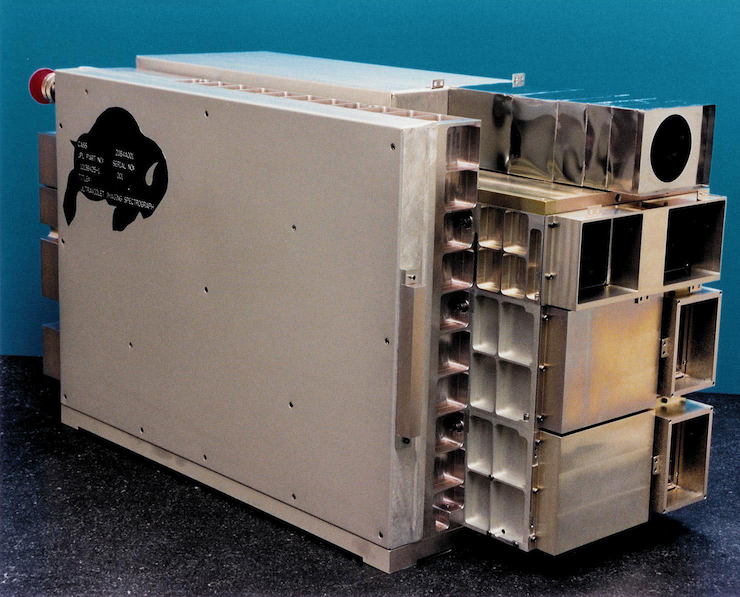
The Ultraviolet Imaging Spectrograph (UVIS) is one of the 12 instruments installed on board Cassini. It was built by the Laboratory for Atmospheric and Space Physics (LASP) located in the Research Park of the University of Colorado in Boulder. UVIS is a set of telescopes used to measure ultraviolet light from the Saturn system’s atmospheres, rings, and surfaces. UVIS also observes the fluctuations of starlight and sunlight as the sun and stars move behind the rings and the atmospheres of Titan and Saturn. These observations are helpful to
better understand the atmospheric composition and photochemistry of Saturn and Titan,
determine the atmospheric concentrations of hydrogen and deuterium in these atmospheres, and
provide information on the nature and history of Saturn’s rings.
UVIS data have also helped to understand the physical properties of the water plumes and the salty ocean inside Enceladus. A detailed description of UVIS can be found in the UVIS Science Team’s paper published in Space Science Reviews Esposito et al., 2004. The following is a brief description of the components of UVIS.
2.2Instrument description
UVIS has two spectrographic channels: the extreme ultraviolet channel (EUV 56 to 118 nm) and the far ultraviolet channel (FUV 110 to 190 nm). The ultraviolet channels are built into weight-relieved aluminum cases, and each contains
a reflecting telescope,
a concave grating spectrometer,
an imaging, pulse-counting detector.
Three slits are available:
a high resolution slit
75 and 100 μm slit width for the FUV and EUV channel, respectively,
a low resolution slit
150 and 200 μm slit width for the FUV and EUV respectively,
an occultation slit of 800 μm width,
identical for both channels.
In both the EUV and the FUV channels the detector is a CODACON (CODed Anode array CONverter), consisting of 1024 pixels in the spectral direction and 64 pixels in the spatial direction.
UVIS also includes
a high-speed photometer channel (HSP),
a hydrogen-deuterium absorption cell channel (HDAC),
an electronic and control subassembly.
2.2.1EUV
The extreme ultraviolet channel (EUV) is used primarily for imaging spectroscopy and spectroscopic measurements of the structure and composition of the atmospheres of Titan and Saturn.
The EUV channel consists of
a telescope with a three-position slit changer,
a baffle system,
a spectrograph with a CODACON microchannel plate detector and associated electronics.
2.2.2Telescope
The telescope consists of
an off-axis section of a parabolic mirror with a focal length of 100 mm,
a 20 x 20 mm aperture.
A precision mechanism positions one of the three entrance slits at the focal plane of the telescope, each translating to a different spectral resolution. The spectrograph uses a toroidal grating that focuses the spectrum onto an imaging microchannel plate detector to achieve both high sensitivity and spatial resolution along the entrance slit.
2.2.2.1Microchannel plate detector
The microchannel plate detector electronics consist of
a low-voltage power supply,
a programmable high-voltage power supply,
charge-sensitive amplifiers,
associated logic.
2.2.2.2Solar occultation port
The EUV channel also contains a solar occultation port to allow solar flux to enter the telescope through a small aperture when the sun is 20 degrees off-axis from the primary telescope.
2.2.3FUV
The far ultraviolet channel (FUV) is used primarily for imaging spectroscopy and spectroscopic measurements of the structure and composition of the
atmospheres of Titan and Saturn,
rings and icy satellites.
The FUV channel is similar to the EUV channel except for the
grating ruling density,
optical coatings,
detector details.
The FUV electronics are similar to those for the EUV except for the addition of a high-voltage power supply for the ion pump.
2.2.4HSP
The high-speed photometer channel (HSP), using a solar blind CsI photocathode, performs high signal-to-noise-ratio stellar occultation measurements of the structure and density of material in the rings, as well as the atmospheres. The HSP resides in its own module and measures light that is focused by its own parabolic mirror with a photomultiplier tube detector. The electronics consist of a pulse-amplifier-discriminator and a fixed-level high- voltage power supply.
2.2.5HDAC
The hydrogen-deuterium absorption cell channel (HDAC) is used to measure the relative abundance of D/H in the Saturn system from their Lyman-alpha emission by using
a hydrogen cell,
a deuterium cell,
a channel electron multiplier (CEM) detector to record photons not absorbed in the cells.
The hydrogen and deuterium cells are resonance absorption cells filled with pure molecular hydrogen and deuterium, respectively. They are located between an objective lens and a detector. Both cells are made of stainless steel coated with teflon and are sealed at each end with MgF windows. The electronics consist of
a pulse-amplifier-discriminator,
a fixed-level high-voltage power supply,
two filament current controllers.
2.2.6Microprocessor
The UVIS microprocessor electronics and control subassembly consists of
input-output elements,
power conditioning,
science data and housekeeping data collection electronics,
microprocessor control elements.
The microprocessor on the UVIS
operates the instrument,
executes various operating modes for data handling and compression,
buffers the instrument’s observation data for pickup by the Cassini Orbiter’s Command and Data Subsystem (CDS).
The Cassini spacecraft points the UVIS telescopes to the desired target (including stars, the Sun, atmospheric features, and the limbs of Saturn and its moons). The spacecraft attitude control allows for slews, steps, or drifts across the target. Generally, these spacecraft motions are executed by commands issued from the spacecraft CDS. Synchronization of the instrument activities with the spacecraft motion is achieved by having the CDS send trigger commands to the UVIS at the correct time. These trigger commands instruct the UVIS to execute actions that have been pre-loaded in the UVIS memory.
The data from the observation are buffered for pickup by the CDS. Two pickup rates are allowed: 32 kbps (for occultations) and 5 kbps (for spectral imaging). UVIS team members generate command sequences for each observation, which are loaded in the UVIS memory using a set of tools known as the Uplink Product Generation System (UPGS). The sequence of internal commands is then submitted to the sequencing team at JPL via the UVIS SOPC (Science Operations and Planning Computer). Using the SOPC and the UVIS GSE (Ground Support Equipment), the UVIS team can also monitor the health of the instrument in near real-time. In addition, the SOPC is used to access the data played back by the spacecraft and stored in the JPL Telemetry Data Server (TDS).
2.2.7Background
Like all observations, the UVIS data contain noises from different sources and anomalies. The Cassini spacecraft is powered by 3 radioisotope thermoelectric generators (RTGs), which use heat from the natural decay of plutonium-238 to generate direct current electricity via thermocouples. The RTGs produce a constant background noise that needs to be subtracted from the UVIS observation. There are other backgrounds that may or may not contribute to the total raw counts; however the RTG background is internal to the spacecraft and must always be dealt with. More descriptions on the handling of RTG background can be found in Chapters UVIS Calibration, Saturn’s Aurora, Rings Spectroscopy Data Reduction, and Reflectance Spectroscopy of Icy Moons and Saturn.
A small light leak allowed undispersed interplanetary H Lyman-α to reach the EUV detector for pixels <720, corresponding to wavelengths shorter than 920 Å. For observations prior to 2007, this creates a background referred to as the “mesa” by the UVIS team. Users of this pre-2007 data should be careful to remove the affected pixels. In 2007 the source of the light leak was identified and it was eliminated from subsequent observations by opening the solar occultation door.
For wavelengths >~1150 Å (EUV pixel 971), another wavelength dependent background arises from internal instrument scattering of H Lyman-α. This contribution to the EUV signal is small below 1170 Å, and is estimated to be less than 7% of the total signal, based on comparisons with a modeled H spectrum Ajello et al., 2005. When all the noise sources are subtracted from the signal, the raw observation is ready for the flatfield calibration and the conversion from the raw counts to physical units. Users can find more information regarding backgrounds, the flatfield correction, and calibration in Chapters UVIS Calibration and Cassini UVIS IPHSURVEY Data.
A population of anomalous pixels exist in the FUV detector (~15% of all detector elements), which are characterized by relatively low and possibly nonlinear responses. These pixels are often referred to as “evil”. Although these anomalous pixels are distributed across the entire FUV detector, they often appear in groups along individual columns. Because of the poorly characterized response of these evil pixels, the UVIS team has decided to eliminate them from analysis. This is implemented by assigning an invalid sensitivity to the calibration matrix for these elements. Users can find how the “evil” pixels are identified and handled in Chapters UVIS Calibration and Saturn’s Aurora. An alternate approach is to average over large enough areas of the detector to minimize the effects. This is described in Section 10.3.
2.3PDS
The Cassini UVIS data are stored in the NASA PDS system. The detailed structure and components of the UVIS data in the PDS are described in Chapter PDS Data Structure. In the current chapter we provide step-by-step instructions on how to find and obtain UVIS data from the PDS with the following 3 examples:
a 2005 observation of Saturn’s aurora
a 2004 observation of the reflected FUV spectrum from Phoebe; and
a 2005 Enceladus occultation observation.
2.3.1Example 1
An observation of Saturn’s aurora was carried out around 03:35 on day 172 of year 2005.
Go to the Cassini UVIS data website
Find COUVIS_0011 in the table called “Temporal coverage of each volume”, which contains the observations taken on day 172. And the available data are listed by the date the observations were carried out.
Open COUVIS_0011/DATA/D2005_172/ (or click the full link here ) and search for data with observation time close to 03:35. Save the following data files and LBL files to your computer:
EUV2005_172_03_35.DAT EUV2005_172_03_35.LBL FUV2005_172_03_35.DAT FUV2005_172_03_35.LBLOpen the LBL files to determine the dimensionality, binning, and windowing of the data:
AXIS_NAME = (BAND, LINE, SAMPLE)
CORE_ITEMS = (1024, 64, 163)
UL_CORNER_LINE = 2
UL_CORNER_BAND = 0
LR_CORNER_LINE = 61
LR_CORNER_BAND = 1023
BAND_BIN = 1
LINE_BIN = 1
This information states that the data consist of 1024 spectral elements, called “bands” (spectral bins) from bin number 0 to 1023 with no spectral binning performed (BAND_BIN=1), in 60 lines (spatial bins) from line number 2 to 61 with no spatial binning performed (LINE_BIN=1), and 163 samples (or records).
The user can select for use any programming language to read and analyze the data. The following example uses IDL to read the data:
data = read_binary( filename, data_dims=[ BAND, LINE, SAMPLE], data_type=12, endian='big' )Here the filename can be either
FUV2005_172_03_35.DATorEUV2005_172_03_35.DAT.The data matrix’s dimensions are (1024, 64, 163). Note that endian keyword is set to
bigbecause the machine used to create the binary file follows big-endian byte ordering. Also note that in IDL, type code 12 refers to a 16-bit unsigned integer ranging from 0 to 65535.Some supporting IDL codes and calibration files can be found on the PDS system associated with the data. For example, the users can go to this link to download
F_FLIGHT_WAVELENGTH.PRO, which can provide the wavelength scale of the data. Figure 1 can be generated by summing all the sample data from lines 2 and 61.
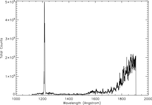
Figure 1:Cassini UVIS observation of Saturn’s aurora on day 172 of year 2005.
2.3.2Example 2
Phoebe observations were made during the flyby around 19:22 on day 163 of year 2004.
Go to the Cassini UVIS data website
Because the data was taken on day 163 of year 2004, find COUVIS_0007 in the table called “Temporal coverage of each volume” and go to
DATA/D2004_163(or click this link to the data folder) and save the following data and LBL files:FUV2004_163_19_22.LBL FUV2004_163_19_22.DATOpen the LBL files to determine the dimensionality, binning, and windowing of the data:
INTEGRATION_DURATION = 30.000 <SECOND>
AXIS_NAME = (BAND, LINE, SAMPLE)
CORE_ITEMS = (1024, 64, 132)
UL_CORNER_LINE = 0
UL_CORNER_BAND = 0
LR_CORNER_LINE = 63
LR_CORNER_BAND = 1023
BAND_BIN = 1
LINE_BIN = 1
This information states that the data consist of 1024 (spectral bins = BANDS) from bin number 0 to 1023 with no spectral binning performed (BAND_BIN=1), 64 lines (spatial bins) from line number 0 to 63 with no spatial binning performed (LINE_BIN=1), and 132 samples (or records). Also note that the integration duration is 30 seconds. This will be useful to convert raw counts into the count rate.
The user can select for use any programming language to read and analyze the data. The following example uses IDL to read the data:
data = read_binary( filename, data_dims=[ BAND, LINE, SAMPLE], data_type=12, endian='big' )Figure 2 can be generated by using the data at sample number 15. Note that to convert the raw counts to the count rate, the users will need to sum all lines, assuming that all lines observed the reflection from Phoebe, and divide the sum by 64x30. The value 30 comes from the 30 second integration duration and the value 64 is the total number of lines used in the observation. See Chapter 8 for more detailed information on the difference between the reflected spectra from Phoebe’s dayside and nightside.
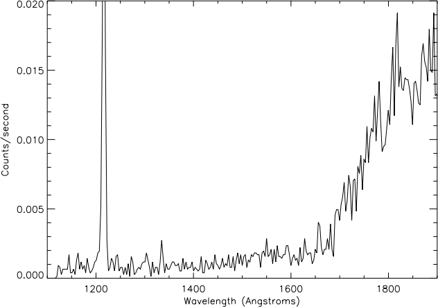
Figure 2:2004 UVIS observation of Phoebe’s dayside.
2.3.3Example 3
An Enceladus occultation observation was carried out around UTC 19:54:56 on July 14th, 2005, which was day 195.
Select COUVIS_0012 which contains the observation data. Then select
DATA/D2005_195. This brings us here. Download the data set containing the closest starting time:FUV2005_195_19_52.DAT FUV2005_195_19_52.LBLOpen the LBL files to determine the dimensionality, binning, and windowing of the data:
AXIS_NAME = (BAND, LINE, SAMPLE)
CORE_ITEMS = (1024, 64, 71)
UL_CORNER_LINE = 19
UL_CORNER_BAND = 0
LR_CORNER_LINE = 43
LR_CORNER_BAND = 1023
BAND_BIN = 2
LINE_BIN = 1
Now we have all the files needed for the 2005 Enceladus occultation observation. Note that the Enceladus observation data is stored in a 3-dimensional array [1024, 64, 71]. As described in the data label, only lines between 19 and 43 contain valid data. And only the first 512 wavelength (band) bins contain valid data because in this particular observation a spectral binning by 2 is carried out.
The user can select to use any programming language to read and analyze the data. The following example uses IDL to read the data:
data = read_binary( filename, data_dims=[ BAND, LINE, SAMPLE],
data_type=12, endian='big' )
Figure 3 can be generated by using the Enceladus data. Note that the users will need to sum all spatial elements (lines) of the corresponding samples in order to obtain the total raw counts as shown in Figure 3.
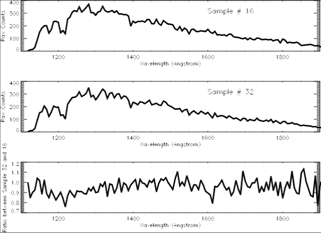
Figure 3:Cassini UVIS observation during the 2005 Enceladus occultation event. The upper panel is the FUV spectrum of the target star at sample record number 16, which is before the occultation. The middle panel corresponds to sample record number 32, during the occultation. The lower panel shows the division between sample 32 and 16, which can be matched with the absorption features of water vapor (see Hansen et al. (2006) ).
In the above, we provide some examples on how different data types can be retrieved from the PDS. The PDS archive contains instructions for reading the data that provide an alternative to the instructions given here. Generally, each COUVIS directory consists of six separate directories:
CALIB
CATALOG
DATA
DOCUMENT
INDEX
SOFTWARE.
These directories contain all the necessary information that is required to read and handle the
data.
The subdirectory SOFTWARE/READERS contains the file READERS_README.TXT that describes how the data can read into IDL.
Basically the file describes an automated procedure that is used to generate a subroutine that reads both the data and calibration files from the appropriate DATA and CALIB subdirectories.
It is important to note that if the reader wants to obtain both the data and the calibration matrix simultaneously with the methods described in the PDS, it will be necessary to download all of the subdirectories and files in the given COUVIS directory.
- Esposito, L. W., Barth, C. A., Colwell, J. E., Lawrence, G. M., McClintock, W. E., Stewart, A. I. A. N. F., Uwe Keller, H., Korth, A., Lauche, H., Festou, M. C., Lane, A. L., Hansen, C. J., Maki, J. N., West, R. A., Jahn, H., Reulke, R., Warlich, K., Shemansky, D. E., & Yung, Y. L. (2004). The Cassini Ultraviolet Imaging Spectrograph Investigation. In C. T. Russell (Ed.), The Cassini-Huygens Mission: Orbiter Remote Sensing Investigations (pp. 299–361). Springer Netherlands. https://doi.org/10.1007/1-4020-3874-7\_5
- Ajello, J. M., Pryor, W., Esposito, L., Stewart, I., McClintock, W., Gustin, J., Grodent, D., Gérard, J.-C., & Clarke, J. T. (2005). The Cassini Campaign observations of the Jupiter aurora by the Ultraviolet Imaging Spectrograph and the Space Telescope Imaging Spectrograph. Icarus, 178(2), 327–345. 10.1016/j.icarus.2005.01.023
- Hansen, C. J., Esposito, L., Stewart, A. I. F., Colwell, J., Hendrix, A., Pryor, W., Shemansky, D., & West, R. (2006). Enceladus’ water vapor plume. Science, 311(5766), 1422–1425. 10.1126/science.1121254