UVIS observations of Saturn and her icy moons are used to derive reflectance spectra as well as images. The techniques are similar for Saturn and for the moons. The satellite surface compositions are dominated by the presence of water ice that has a strong absorption edge near 165 nm. Mapping the strength and location of this absorption edge allows the UVIS data to be used in determining water ice concentrations and grain sizes, as well as probing non-water ice constituents.
The types of UVIS icy satellite observations and their instrument setups are shown in Table 1. In determining icy satellite surface reflectances, the primary observations are the ICYLONs and ICYMAPs, so we focus here on those data, from the FUV channel. ICYLON observations have historically had the focus of building up phase angle and longitudinal coverage of the moons. ICYMAP observations have generally been used for close-in observations during close flybys. The number of rows returned in each observation depends on the data volume available; this varied from observation to observation. ICYEXO analysis is discussed in Chapter Cassini UVIS Ring and Icy Satellite Stellar Occultation Data.
Table 1:UVIS Icy Satellite Instrument Configurations
Configuration | Slit | Integration Time | Channels | Use |
|---|---|---|---|---|
ICYLON | Low res (1.5 mrad) | 120 sec | FUV, EUV | Longitudinal and phase coverage |
ICYMAP | High res (0.75 mrad) | 30 sec | FUV, EUV | Close flyby coverage |
ICYSTARE | Low res (1.5 mrad) | 120 sec | FUV, EUV | Distant observations |
ICYECL | Low res (1.5 mrad) | 120 sec | FUV, EUV | Distant eclipse observations |
ICYPLU | Low res (1.5 mrad) | 180 sec | FUV, EUV | Plume observations |
ICYEXO, ICYOCC | Low res (1.5 mrad) | 5 sec | FUV, HSP | Stellar occultations (see section 6.4 for analysis steps) |
LOPHASE | Low res (1.5 mrad) | 120 sec | FUV, EUV | Longitudinal and phase coverage |
The treatment of UVIS observations of the reflectances of the icy Saturnian moons can be distributed generally into two broad areas, depending on whether the observation is disk-resolved or whole-disk. If the body is distant enough that it is sub-pixel (i.e., smaller than the width of the slit, usually 1.5 mrad), so UVIS sees the whole-disk (Figure 8.1), then it is a “stare” type observation, where the optical remote sensing (ORS) slits are held steady on the body for the duration of the observation. For these observations, if a pointing vector other than UVIS_FUV was used, then the body is not centered in the UVIS slit. In this case, the body may or may not be entirely within the UVIS slit; sometimes the body is only partly within the slit, making the observation of limited value in terms of deriving surface reflectance. If the body is close enough that it is larger than the width of the UVIS slit, it is a disk-resolved observation (Figure 8.2) and there may have been a scan performed across the body, or a mosaic (usually an ISS rider observation), where the slit is positioned in particular locations throughout the observation. Nearly all stare observations are in the ICYLON class. Scans and mosaics may be ICYMAP (usually very close) or ICYLON. LOPHASE observations are distant, disk-integrated observations that use the ICYLON instrument setup while covering particularly low phase angles.
The UVIS instrument measures spectral radiance (units of kR/Å) in each spatial row (1 kR is equal to ). The reflectance is defined as
where P is the calibrated signal from the body with background subtracted, in kR/Å. The solar flux is denoted by S, where S = π F.
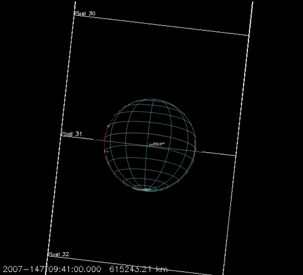
Figure 1:Example of a disk-integrated observation; Enceladus is sub-pixel (0.8 mrad).
If the body is sub-pixel, we must carefully determine the filling factor, the percentage of the pixel filled by the body. This involves using reconstructed kernels to get the distance to the body. The filling factor is
where the body radius is used to determine its size and the pixel size is projected onto the sky at the distance of the body. We divide Eq. (1) by the filling factor Eq. (2) to determine the whole-disk reflectance.
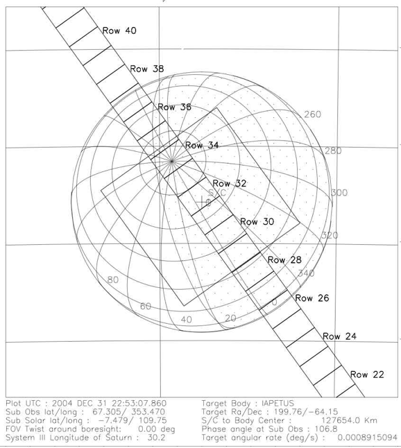
Figure 2:Example of a disk-resolved observation where UVIS was staring at (rather than scanning across) Iapetus. The UVIS low-resolution slit is shown, along with the ISS narrow angle camera (NAC).
The calibration step can be performed before or after background subtraction and
involves the use of IDL routines feuv_reader to open and read the data files and
Get_FUV_2013_Lab_Calibration to generate the calibration array for the date of the
observation. These routines are available on the PDS. The reader is referred to Chapter UVIS Calibration for additional information on reading and calibrating UVIS data files.
9.1Background subtraction 
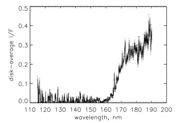
The measured spectrum includes not only the reflected solar signal from a satellite’s surface, but background sources such as RTG noise and interplanetary Ly-α. We must subtract out this background signal before dividing by the solar spectrum when determining the reflectance spectrum. For a background spectrum we use (when possible) a night side spectrum obtained during the same time period as the dayside spectrum. It is not always possible to use a night side spectrum, so often we use an off-body spectrum. A night side spectrum is preferable so that we can obtain a reflectance value at Ly-α. Because the dark-sky Ly-α signal is higher than the reflectance from the surfaces of the icy moons, we cannot subtract off the background and obtain a reasonable Ly-α albedo. The nightside signal includes RTG noise as well as reflected Saturn system Ly-α. The contribution from interplanetary Ly-α, to both the day and night sides, is negligible compared to solar Ly-α. Thus the only difference between the day and night signals is the reflected solar spectrum. Figure 8.3a shows a background spectrum displayed along with Phoebe’s reflected solar spectrum; even at the shorter wavelengths where the signal is low, the Phoebe signal is above the background level in this observation. For the nightside data, we looped through the data and chose rows/times when the incidence angle was greater than 100 deg.
Sample spectra from Phoebe (phase angle = 42°):
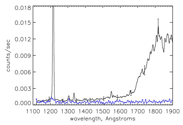
Average raw spectrum (counts/s) from the dayside (average of 1224 spectra) and nightside background spectrum (in blue), with sample statistical error bars shown.
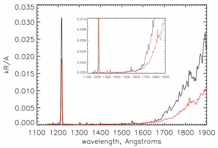
Average calibrated spectrum (kR/Å), nightside background subtracted, with scaled solar spectrum overplotted (in red). The solar spectrum has been scaled by fitting to the reflected 1335 Å C II feature in the Phoebe spectrum.
9.2Solar spectrum division 
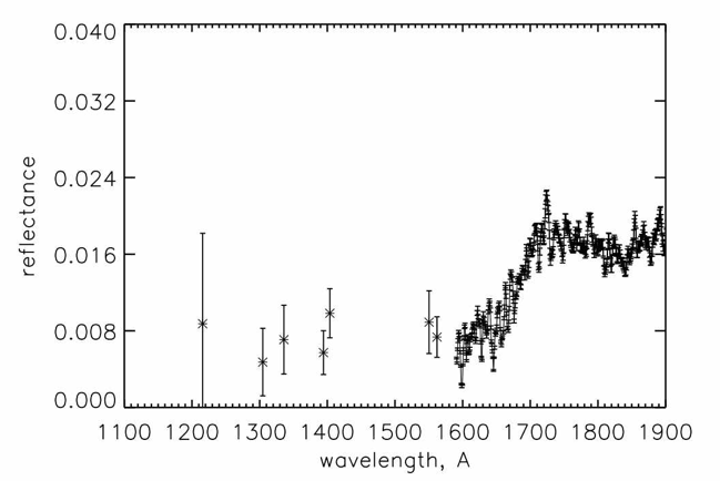
We use the solar data as measured by SOLSTICE on the SORCE spacecraft (McClintock et al., 2000), scaled to the heliocentric distance of Saturn on the day of the observation, making sure to use the solar spectrum for the sub-solar longitude appropriate for the UVIS observation. (We use the solar spectrum measured at Earth but adjusted forward or backward in time to account for the difference between the sub-solar longitudes facing Earth and facing Saturn on the day of the observation.) See Figure 8.3b for a sample Phoebe spectrum compared with a scaled solar spectrum. The solar flux decreases dramatically below ~1500 Å, and in addition, the reflectance of water ice is very dark at wavelengths <1650 Å. The combination of these two effects means that the icy moons generally do not reflect very much light at the shorter FUV wavelengths, and as a result, the signal is extremely low. The resultant reflectance continuum is noisy, so we often choose to create binned reflectance values at the wavelengths where the satellite spectrum exhibits reflected solar lines such as the carbon line at 1335 Å (see for instance Figure 5). Figure 6 is an example reflectance spectrum showing division by the solar continuum.
9.3Saturn reflectance spectra 
Sample reflectance spectra::
The goals and methods for Saturn science are similar to those for the icy satellites. The reflected intensity (I/F) contains information on a few hydrocarbons (principally acetylene) and the scattering and absorbing properties of haze. Most of the Saturn data obtained with UVIS as the prime instrument are named EUVFUV in the observation ID. These are image cubes, where the slit was scanned across the disk of Saturn resulting in two spatial dimensions and one spectral dimension. The scan stops at many places to allow other instruments to image, then continues to build up a complete image. Viewing and lighting geometry information is needed to interpret the data. The required geometry consists of view and emission angles of the outgoing and incoming photons relative to the local zenith direction, and the phase angle (angle between incoming and outgoing rays). The following list is an example of step-by-step instructions for a user wishing to calibrate the UVIS data and obtain the geometry needed to interpret the data.
Download new EUVFUV (or other data) files from the data repository.
Create a list of file names if there are multiple files in a data set. This is just a text file with a list of all the file names going into the cube program.
Download applicable SPICE kernels, corresponding to the days of the observations, from the Cassini NAIF kernel repository
Compile (currently IDL) and then run
cube_generator.pro(see Chapter Cube Generator) (substitute your own directory pointers – the following are examples)Input files and input batch files are located in the directory
/dst/SaturnFUV/RawData/or/dst/TitanFUV/RawData/.Output should be the default,
improvedoutput file format. Save the output file in the folder /CalibratedData/ found either in /dst/SaturnFUV/ or /dst/TitanFUV. The filename must match the syntax of the files already in those folders.Use
LTaberrationCheck RTG correction (and use default value of 0.0004 counts/second/pixel)
Select
Saturnfor target body.Use the default
full calibration and flatfielding sequence.Kernels and kernel batch files are located in the folder
/Kernels/.Once all the above is entered, click “Create.” Note that for some datasets, correct kernels still generate a kernel error because of holes in the kernels. If an error is encountered, check to see that “loaded kernels” all match date of observation, then check “override kernel checks” and click “Create” again.
Calibrate to I/F by division by a solar spectrum as described above. Alternately one can run a ‘forward calculation’ as described elsewhere in this document (see Chapter UVIS EUV/FUV Channel Saturn and Titan Occultation Reduction) to estimate instrument count rates given a model intensity spectrum, and compare the simulated counts with observed counts.
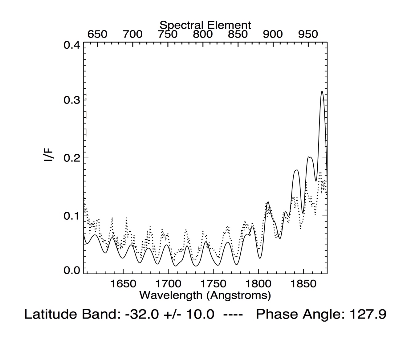
Sample Saturn spectrum. I is the measured intensity; πF is the incidence solar flux.