13.1Introduction 
Cube Generator (CG) is an IDL widget to read and process raw Cassini UVIS data files, and combine the processed data with geometric parameters as calculated by Josh Colwell’s Geometer Engine into an Image Cube for use in further investigations. Users are given a variety of options regarding the processing of the data and geometer options. This document provides a reference and tutorial for new users to CG. After a brief introduction and comments regarding the installation and compiling of CG, the tutorial is ritten in the order a typical user would use to create an image cube from raw data.
13.2Installation 
All the necessary files needed to run CG are available on the planetary data system (PDS). Unzip, or save, all the included files to a single directory. Cube Generator will look for the files it needs locally. Many of the files within the CG package are either modified or unmodified versions of code written by other members of the UVIS science team. They have been renamed to avoid confusion or conflict with previously extant code.
13.3The Interface 
Cube Generator requires at least IDL 5.5 and the ICY spice interface, available from
ftp://
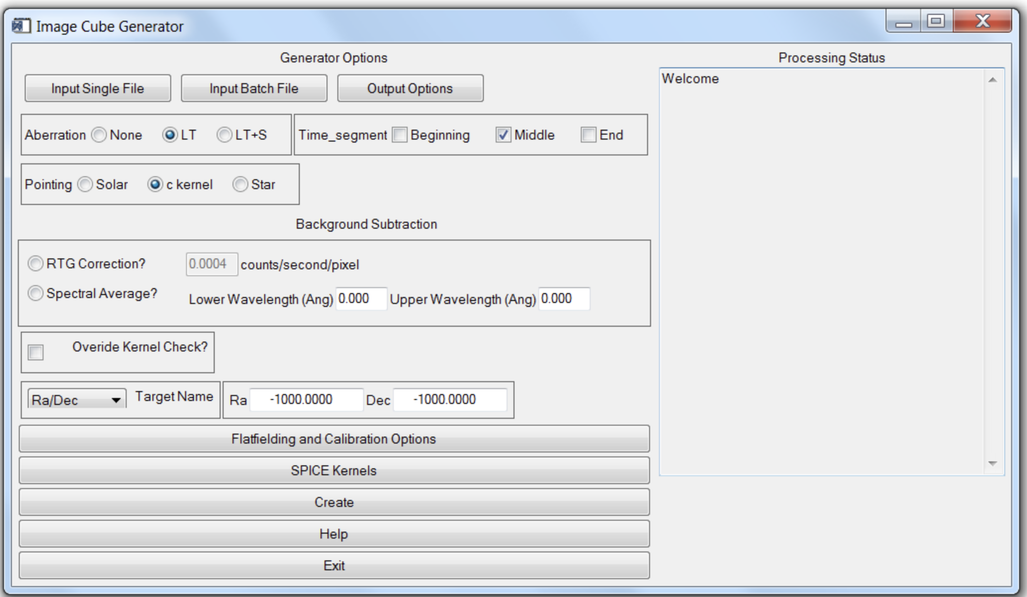
Figure 1:Base level menu for Cube Generator.
On the left half of the widget, a series of inputs and menu buttons provide access to the various options that will be discussed in detail in the rest of this document. The text block on the right will update as the widget is used with confirmation and status messages for the user. When the image cube is created, it will also contain a running summary of program steps, status messages, and any errors that may occur.
13.4Raw Data Input 
Raw data files exist on the PDS independent of Cube Generator. A user may input raw data downloaded from the PDS in two ways, either as a single data file from or as a list of files that will be combined to form a single output cube (as in the case of an observation that has been split into multiple raw data files). For any data files obtained from the PDS, the accompanying label file must be downloaded and placed in the same directory as the data file. To create an image cube from a single data file, simply click on the ‘Input Single File’ button. A file selection dialog will open allowing the user to navigate to where the file is saved on their computer and select it for input.
In the case of an observation that consists of more than one raw file, the user will select the ‘Input Batch File’ button. The program is asking for a text file that lists the names of all the data files to be combined into a single cube in the order they are listed in the file. Cube Generator does not sort files should they be listed out of temporal order, though such an instance would not impact the validity of the associated geometric data. Currently, the only option for entering a series of data files for batch mode is in the form of a text file.
13.5Output Formats 
Selecting the ‘Output Formats’ button will change the menu options on the left half of the Cube Generator widget as follows (see Figure 2).
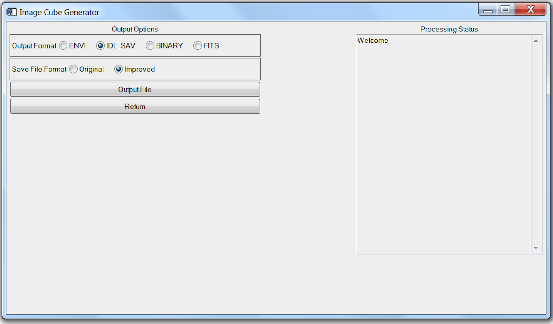
Figure 2:File Output options menu
Users have the option of outputting the image cube in four basic formats; ‘Envi’, ‘IDL_SAV’, ‘Binary’, and FITS. The default setting an IDL save file (IDL_SAV) which will save the cube as an IDL structure that can be restored at a later time for further use. If the IDL_SAV output format is selected, there is a further option of the ‘Original’ or ‘Improved’ file format. The ‘Original’ format is included for those users who have already written code that accepts image cubes. The ‘Improved’ format was designed by Josh Colwell to eliminate the need to reset an IDL session after the creation of each cube due to changing structure dimensions. It is strongly suggested that users create cubes in the ‘Improved’ format. For further details on the structure of both the ‘Original’ and ‘Improved’ save file formats, see Appendix 1 at the end of the document.
The ‘ENVI’ output format creates an image cube and associated header that can be read by the ENVI image processing package. ENVI is an IDL extension that must be purchased separately from ITT.
Finally, the ‘Binary’ output format is simply a binary array of double float values. Note that there is no information in the Binary format to inform a user as to the dimensions of the included data.
The ‘Output File’ button will open a selection dialog that allows the user to select the name and location where the image cube will be written. When the user has selected the output format and file names, press return to change the menu back to the base screen (Figure 12.1).
13.6Main Menu Options 
Back at the base level menu, the user has a few options that relate to the calculation of the geometric parameters or the processing of the raw data. These options are generally left at their default state, though some special cases may require their modification.
First, the boxed sub-menu labeled ‘Aberation’. This option affects how Geometer will calculate the geometric parameters. The default setting of ‘LT’ commands geometer to calculate the state variables as corrected for light-time. ‘None’ does not correct for light-time and ‘LT+S’ corrects for light-time and stellar aberrations. For many observations, the difference between aberration states would likely be negligible. However, given the possible non-negligible effect on some calculations, the ‘LT’ correction is set as default.
To the right of the aberration box is the time segment box. Users may select any combination of three discrete times within an integration period to retrieve geometry. “Beginning” is at the start of the integration period, “Middle” is at half of an integration period, and “End” is at the end of the integration period. By default the “Middle” button is preselected. For each time period, a separate structure will be returned, denoted by “datastruct2_initial, datastruct2, and datastruct2_final, for the three time periods, with geometry within each for the selected time periods. If a time period is not selected, then that particular structure contains a zero.
Below the aberration selection menu is a box used to select the pointing reference, which may be Solar, c kernel (the default setting), or Star. In the case of Solar or Star the pointing of the instrument is referenced to the vector between the instrument and either the Sun or a star. If “Star” is selected an input box appears requiring that the name of the star be entered.
Below the pointing box is a check-box that allows the user to select between two types of background subtraction, RTG or spectral average. If RTG is selected, the text box will become active and, if the user chooses, a new RTG noise value may be entered. Cube Generator will subtract from each pixel an RTG noise level based on this value and the integration length of each observation record. If a new RTG correction value is entered, the user MUST press return for IDL to record the new value. If “Spectral Average” is selected the user must enter upper and lower spectral bounds, which results in the average of the raw counts over that spectral interval to be subtracted from the raw counts.
Below the “Background Subtraction” box lies another check-box labeled ‘Override Kernel Check?’. If selected, this will force CG to continue and make an image cube despite errors from the called SPICE routines that indicate insufficient kernel data to calculate geometric information. Generally, it is in the users interest to allow C-kernel errors to interrupt CG, however there are some cases in which an error may be ignored.
Below the “Override Kernel Check” is a pull down ‘Target Name’ menu, as shown in Figure 3. The user is required to manually select the Target relative to which Geometer will calculate the relevant parameters. If no target is selected (or the Ra/Dec target is selected without changing the values to the right), CG will declare an error and interrupt the image cube creation process. If the user wants to calculate parameters relative to a fixed Ra/Dec value, select Ra/Dec as the target and modify the values to the right of the pull down menu (remembering to hit return in each field to register the changes with IDL).
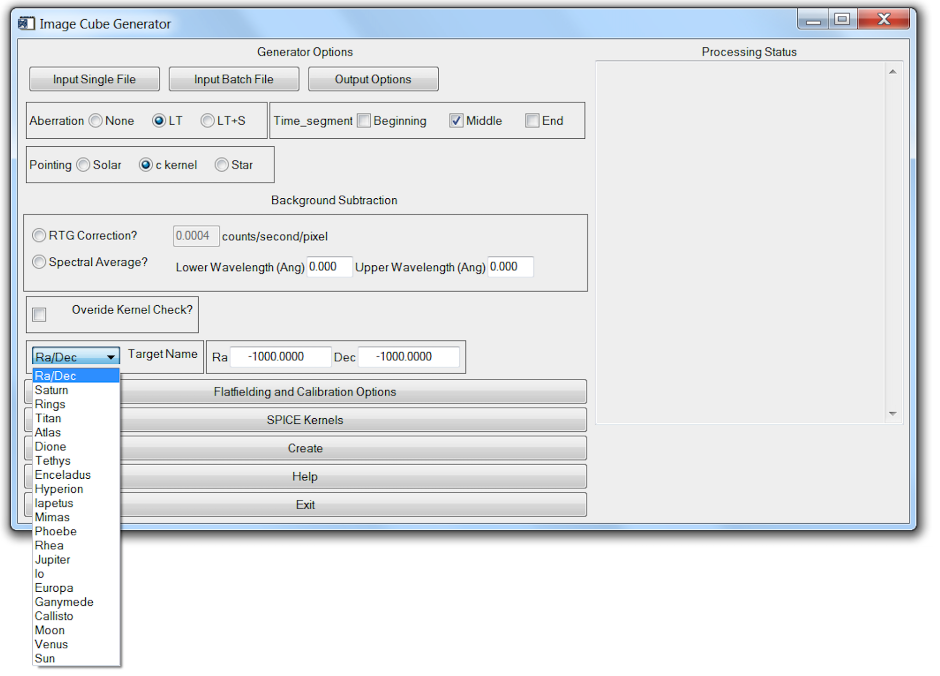
Figure 3:Target Name pull-down menu.
13.7Flatfielding Options 
For general use, this menu (Figure 4) will not need to be accessed. The default setting will process the raw data according to the team-sponsored procedure. The default processing scheme corrects the raw data by the following steps.
Calibration using calibration factor temporally interpolated to time of observation.
Apply Red Patch (for FUV data only).
Apply Andrew Steffl (AJS) Not-a-Number (NaN) flatfield with 1.05 multiplicative modifier.
Interpolate across NaN pixel gaps.
Export corrected data.
Should a user want to eliminate of modify any of the steps above, the Ala Carte menu exists to allow flexibility and is accessed by deselecting the ‘Full Flatfielding Routine’ in Figure 4.
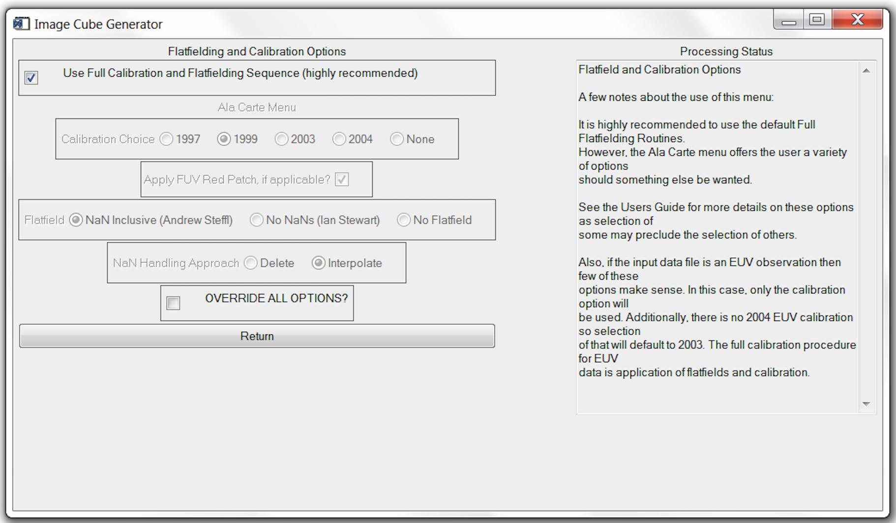
Figure 4:Flatfielding Processing Menu
The Ala Carte flatfielding menu allows the user to select which ground calibration to apply, 1997, 1999, 2003, or 2004, whether to apply the Red Patch, how to handle NaN’s, and which flatfield to use. The calibration and flatfields both have the multiplicative modifiers applied to them.
Some options within the Ala Carte menu preclude other selections. For instance, selection of the “No NaNs (Ian Stewart)” flatfield will override the user’s selection of a ‘NaN Handling Approach’ as those selections no longer have any meaning. Similarly, choosing to apply no calibration will automatically disable the FUV Red Patch, regardless of whether the patch was selected to be applied by the user from the Flatfielding menu.
Each of the choices under the ‘Calibration Choice’ refer to the year of a lab calibration. If the 1999 lab calibration (the default setting) is selected, and the inputted data set is an FUV observation, the derived correction factor of 0.91 is applied automatically. Selection of any of the other calibrations WILL NOT have a correction factor applied.
If the user checks the box next to the ‘Override all Options?’ label, NO calibrations or flatfields will be applied to the data. The output in this case would be simply raw data and the geometric information.
13.8SPICE Kernels 
The SPICE Kernel Options menu (Figure 5) provides a series of tools to manage the SPICE kernels accessed by Geometer to calculate the geometric parameters included in the image cube. SPICE kernels loaded into memory via the ICY routines stay resident in memory until IDL is shut down. Resetting the IDL session DOES NOT clear SPICE kernels from memory. Thus, when processing a large number of files, it is possible to have many, and possibly conflicting, kernels loaded.
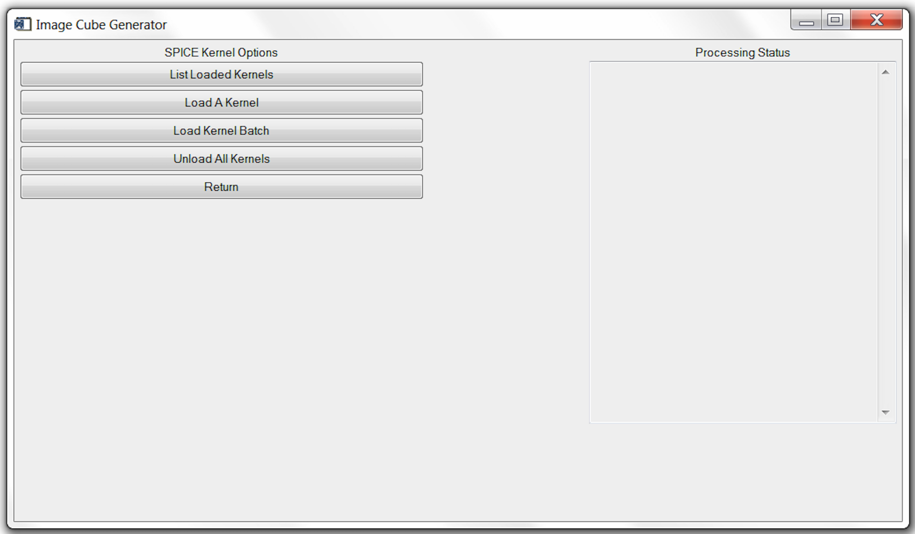
Figure 5:SPICE Kernel Options menu.
The first option in this menu will list all the SPICE kernels currently in memory in the right hand text box. This is useful for when CG aborts due to a C-kernel error. Examining the loaded kernels may identify the missing kernel.
To load a single kernel into memory, user the ‘Load a Kernel’ button. A file selection dialog will open and, if successful, the Processing Status box will confirm loading of the kernel. The user may also load a series of kernels simultaneously via the ‘Load Kernel Batch’ button. Similar to the batch loading function for raw data files, this batch load asks for a text file that contains the paths and names of the desired kernels. And, as with the single kernel file loading option, a successful operation will be indicated in the status box. Alternatively the user may choose to load spice kernels independently of Cube Generator as long as the kernels are loaded into the numerical processing software (e.g., IDL) before running Cube Generator.
Finally, the ‘Unload All Kernels’ button will force IDL to clear all SPICE kernels from memory. If you are concerned that the wrong kernel might be used to calculate the geometry, use this to clear memory and then re-load the specific kernels you want to use.
A quick note about the loading of SPICE kernels. The ICY interface requires that the first kernel in memory be the leap second correction kernel (LSK). Thus, when loading, make sure that is either the first loaded or the first entry in the text batch file. In addition, the latest loaded SPICE kernels take precedence. Thus, if two kernels are loaded that cover overlapping times, the latter will be used to calculate state variables. The user should use the ‘List Loaded Kernel’ and ‘Unload All Kernels’ functions to ensure kernels are loaded in the right order for the appropriate data file.
13.9Cube Creation 
Finally, once all the variables and options have been set as above, pressing the ‘Create’ button creates the image cube. As the code runs, the ‘Processing Status’ box will update. If there are any errors during processing, an appropriate message will be displayed and instruct the user in how to correct the problem. On success, the output file location and dimensions will be displayed.
13.10Final Menu Options 
At the base level menu, there are two final buttons that haven’t been described. Both are so self-explanatory that they shouldn’t require any mention, but to be insanely complete, a few words.
‘Help’ opens an abridged version of this document within the widget framework for quick reference as needed.
‘Exit’ exits.
13.11Examples of Restoring the Contents of Variables 
Suppose that one needs to look at the calibrated data, denoted by the variable name “UVIS” and compare this to the pixel center longitude determined at the middle of the integration period. In IDL the code would be written as follows:
Restore,filename
UVIS = datastruct2.UVIS
Pixel_center_longitude = datastruct2.pixel_center_longitude
Alternatively suppose one needs to look at the raw counts and compare this to the pixel center phase angle for geometry determined at the beginning of the integration period. In IDL the code would be as follows:
Restore,filename
Rawcounts = datastruct2_initial.rawcounts
Pixel_center_phase_angle = datastruct2_initial.pixel_center_phase_angle
By default, the number of spatial pixels is 64 and the number of spectral pixels is 1024. However observations do not always make use of all of the spatial or spectral pixels depending on data volume restrictions. Therefore although the size of the UVIS or raw counts array are 64 X 1024 X number of data records, only pixels that were used in data acquisition will contain non-zero values. This may be determined by the variables XMIN, XMAX, YMIN, and YMAX. Furthermore pixels may be binned on board the spacecraft before and will also affect the number of non-zero pixels. This may be determined by the variables XBIN and YBIN. Some variables are independent of the pixels on the detector, e.g. “SPACECRAFT_LONGITUDE”. Thus the size of this array will be 1 X the number of data records.